1.0 Introduction

Mechanical Design and Analysis accounts for approximately 9 to 14 questions on the Mechanical FE exam. This makes Mechanical Design and Analysis tied for second as the Sections with the most possible problems on the FE exam. This section primarily focuses on machine design mechanical components like springs, pressure vessels, beams, piping, bearings, power screws and transmissions. In addition, other topics that support machine design mechanical components are discussed in this section, like manufacturability, quality, and reliability. Then this section switches to topics that are common in Thermal & Fluids like hydraulics, pneumatics and electromechanical components. Finally, this section repeats topics like beams, piping, stress analysis, deformation, stiffness that are covered in previous sections. This section will point you to the correct section when these repeat topics are discussed.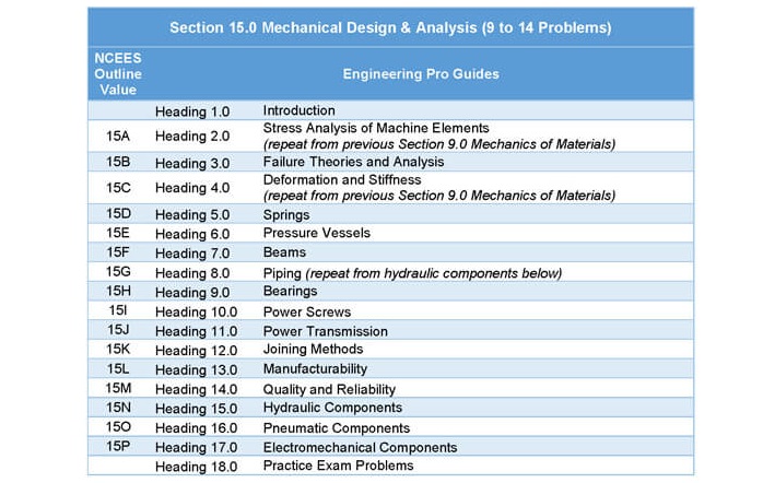

2.0 Stress Analysis of Machine Elements

Stress analysis of machine elements is discussed in Section 9.0 Mechanics of Materials, there are many topics within that section that discuss the stress for all possible types of loads.

3.0 Failure Theories and Analysis

Failure can mean a component has been completely fractured; permanently distorted or its function has been compromised. In Section 10.0 Material Properties and Processing, various strengths of material properties have been presented. Unfortunately, these strengths which can be used to determine the stress levels at which failure will occur apply only to simple loadings like tension, compression or shear that occurs in one axis. In real life situations and for most of the FE exam, the simple loadings can be assumed. However, there may be a couple of questions on the FE exam where there are complex loadings. For these questions you need to use one of the following failure theories, (1) Maximum Normal Stress Theory for Brittle Materials, (2) Mohr’s Theory for Brittle Materials, (3) Maximum Shear Stress Theory for Ductile Materials and (4) Distortion Energy Theory for Ductile Materials also known as Von Mises Theory.

...

This topic is covered in the practice exam and technical study guide, see the link below.

4.0 Deformation and Stiffness

Deformation and stiffness is covered in Section 9.0 Mechanics of Materials, there is another topic within that section called deformations. In addition, Section 10.0 Material Properties and Processing has a section on the physical properties of materials like stiffness.

5.0 Springs

The topic of springs was initially discussed in Section 6.0 Vibration, but it is reintroduced in the section with an emphasis on applications. A spring provides an opposing force that is dependent on the stiffness of the spring and the deflection of the spring from its free length.

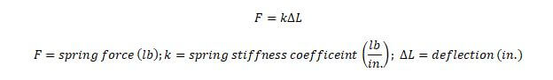
If the spring is not deflected then it is at its free length. The spring force at a deflection of 0 will be equal to zero. When a spring is deflected at a design or operating load, then the force will be found using the previous equation. If the spring is fully deflected, then it is at its maximum load. This full deflection amount is often called solid length.

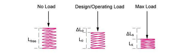
Figure 5: A spring's force is corresponds to the level of deflection.

The springs topic continues in the technical study guide with different types of springs, force analysis and fatigue analysis.

6.0 Pressure Vessels

A pressure vessel is a container designed to hold gases or liquids at a pressure substantially higher than ambient pressure. In Machine Design, pressure vessels are used to hold compressed air or hydraulic fluid.

Pressure vessels are used to store both gases and liquids. Pressure vessels can come in a mixture of spherical and cylindrical shapes and these vessels can have thick or thin walls. The primary pressure vessels that you should know are the thin wall pressure vessels, but thick wall pressure vessels are also on the NCEES Machine Design outline.

Typical questions on the FE exam may include finding stresses or designing pressure relief valves. The stresses within the pressure vessel can be one of three types, (1) hoop stress, (2) longitudinal stress or (3) radial stress.

Figure 1: A pressure vessel will experience internal pressure due to the compressed fluid. This will result in stresses in the material in both the longitudinal direction and also in the tangential direction.

(1) Hoop Stress: Hoop stress can also be called tangential stress. This is the stress that is tangent to the surface of the pressure vessel.

(2) Longitudinal Stress: The longitudinal stress is sometimes called axial stress. This stress is parallel with the axis of the pressure vessel. This stress creates tension in the longitudinal direction.

(3) Radial Stress: Radial stress is the stress that pushes perpendicular against the surface of the pressure vessel from the inside. This would be equivalent to the internal pressure of the liquid or gas within the pressure vessel.

Thin vs. Thick Wall

The thin walled pressure vessels make calculations easier. A thin walled pressure vessel is defined as having a ratio of radius to thickness as greater than 10.

A thin walled pressure vessel uses membrane theory, which assumes that the hoop stress in the thickness of the wall does not vary. The hoop stress within the thickness of the wall is constant from the outside of the wall to the inside of the wall.

Design Factor

A design factor is a factor of safety that is applied to the design of the pressure vessel. In engineering practice, you do not design a pressure vessel at its design pressure, you typically provide a factor of safety to ensure that the pressure vessel is designed to withstand much more than the expected stresses in the pressure vessel.

Materials

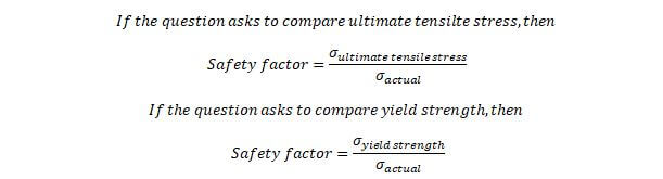
The pressure vessel stresses should be designed well below the maximum allowable stresses of the pressure vessel material. For the exam, you should have the following material properties readily available.

• Ultimate tensile strength or tensile strength: The maximum stress before failure.
• Yield strength: The maximum stress before permanent deformation occurs.

Spherical vs. Cylindrical

The two main pressure vessel shapes in Machine Design are spherical and cylindrical. The hoop stress for these pressure vessels will be dependent on the internal pressure (assuming no external pressure), radius and thickness. These equations only work if the pressure vessel qualifies as a thin walled pressure vessel.

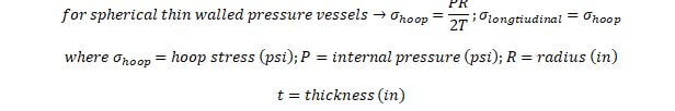
The hoop stress is typically the design criteria for pressure vessels, since this stress is much higher than the internal pressure and is twice the longitudinal stress for cylindrical pressure vessels. The hoop stress and the longitudinal stress are equal to one another because stresses are the same in all direction for spheres. There is no longitudinal axis in a sphere.

Thick Wall Theory

If you encounter a thick wall pressure vessel, then you cannot use the previous equations. You must use the following Thick Wall Theory equations. These equations show that the stress in the thickness of the wall of the pressure vessel will vary based on the location that stress is measured within the wall thickness.

The hoop stress and radial stress will vary based on location “r”.

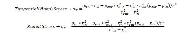
The sum of the hoop stress and the tangential stress will be constant and independent of location “r”.

The longitudinal stress is also independent of location “r”.

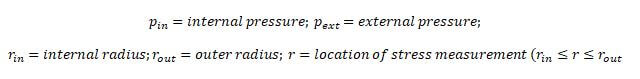
When there is only internal pressure then the critical condition will occur when location “r” is equal to the internal radius of the pressure vessel. If you substitute the external pressure as zero, then the hoop stress equation reduces to the following.

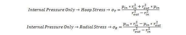
In Machine Design, typically pressure vessels are only subject to internal pressures. However, you should be able to deduce the equations for external pressure only with the critical condition occurring at the outer radius.

This topic is covered in the practice exam and technical study guide, see the link below.

7.0 Beams

This topic is covered in the practice exam and technical study guide, see the link below.

8.0 Piping

This topic is covered in the practice exam and technical study guide, see the link below.

9.0 Bearings

Bearings are used to separate two components, while permitting relative motion between the two components. Bearings are designed to have very little friction and often have a lubricant between the bearing and the components.

There are two main types of bearings, plain surface bearings and rolling contact bearings. A rolling contact bearing consists of either a ball or roller between the two components. A plain surface or sliding bearing or journal bearing consists of a bearing surface and no rolling elements. This is common of a shaft rotating within a bushing. This is a housing that sits around a shaft that provides a bearing surface. The FE exam will most likely focus on the rolling contact bearings and the lubrication of plain surface bearings. Each type of bearing has sub-types as shown in the figure below.

In the Machine Design field, the two types of bearings each have their own typical design questions that can occur on the FE exam. For roller contact bearings, typical questions focus on the load and life of the bearing. In application, you will encounter bearings that have a rated load and rated life. You will have to interpret this information and apply it to your situation. This typical process will be discussed in the life-load analysis.

For plain surface bearings, you must analyze the lubricant that is used. You must determine the appropriate lubricant based on viscosity, temperature and you must also determine the amount of clearance between the two components. This will be discussed in Lubrication Analysis.

Lubrication Analysis

Lubrication analysis is based on finding the correct type of lubrication, viscosity, temperature and amount to properly suit the design of the plain bearing or journal bearing. This analysis is not normally used for roller-contact bearings. The most common type of lubrication is called boundary lubrication. In this type, the lubrication provides a microscopic thin layer between the two moving components. The following bearing characteristic number also known as the Sommerfeld number is a dimensionless number that is used in selecting the properties of the lubricant.

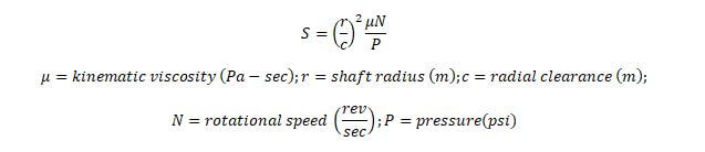
The radial clearance is the clearance between the shaft and the bushing. The pressure is the force per area that the shaft imparts on the lubricant. Since the shaft is cylindrical, the pressure can be found through the following equation, where r is the radius of the shaft and L is the length of the shaft.

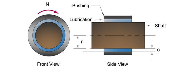
Figure 2: The bearing characteristic number is based on the radius of the shaft, the clearance between the shaft and the bushing, the viscosity of the lubrication fluid, the rotational speed of the shaft and the pressure of the shaft on the lubricant.

The Sommerfeld number is mostly determined by the shaft speed (N), shaft weight (W), shaft dimensions (D, L) and the shaft fit (c). In lubrication analysis, you must select the appropriate lubricant, which will determine the viscosity value. The SAE and lubrication manufacturers publish lubricant graphs that look like the one below. These graphs show the relationship between viscosity and temperature. As the temperature increases, the viscosity decreases. When selecting a lubricant you should pay attention to its operating temperature and choose one of sufficient viscosity for the applicable operating temperature.

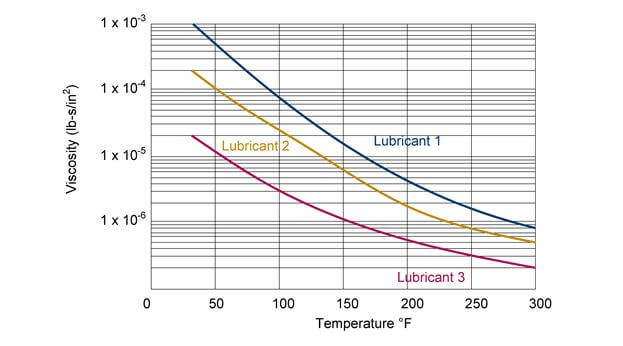
Figure 3: The viscosity of a lubricant will decrease as temperature increases.

Once you have selected the lubricant and found the viscosity that corresponds to the operating temperature, then you can determine the Sommerfeld number. This number and the L/d ratio of the shaft will then determine the minimum film thickness through graphs that look like the next figure.

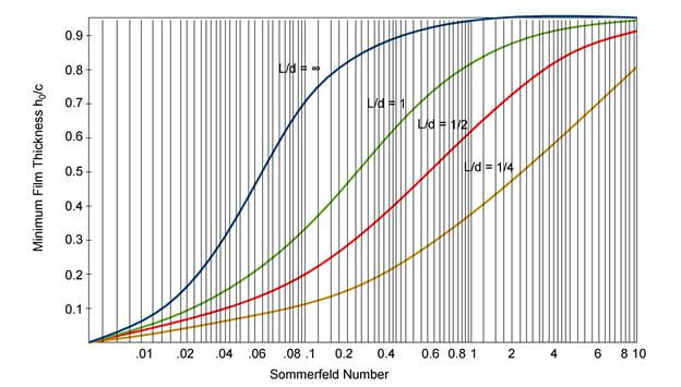
Figure 4: Once you have found the Sommerfeld number then you can use a similar graph to find the minimum film thickness.

The term h0 is the minimum film thickness and c is the clearance that was previously determined by the shaft fit. The minimum film thickness is typically designed to be greater than the roughness. If the surface roughness of the components is greater than the minimum film thickness of the lubricant, then the lubricant will not protect the surface of the components and the components will degrade. If you do not have adequate minimum film thickness then you may have to select a different lubricant with a greater viscosity, however there is a tradeoff between the viscosity and the amount of friction that is created by the lubrication. These two opposing qualities of a lubricant make the process of selecting a lubricant difficult. However, for the purposes of the exam you should just be familiar with the steps in this process. It is most likely that a question in this area will only focus on one step, since there is only 6 minutes available to complete a problem.

Life Load Analysis

The life load analysis topic under the NCEES outline primarily refers to roller contact bearings, since these bearings will fail due to fatigue and their life is dependent on the load. The basic equation that you must use for life-load analysis type questions for ball bearings is as shown below. The life of a ball bearing varies by the cubed of the load. This means that if the load on a ball bearing is doubled, then the life of the ball bearing compared to the original life is cut by 1/8th.

Roller bearings have a different ratio from ball bearings. These roller bearings are cylindrical or needle type bearings.

Roller contact bearing manufacturers provide data for the load, rating life, life, median life, basic load rating, etc. The rating life is the life at which 10% of bearings have failed and is shown as the variable, L10. Life is determined as the number of revolutions the roller bearing can withstand prior to showing signs of fatigue. The median life is the life at which 50% of the bearing have failed and is shown as the variable, L50. These life values are given as a function of the rated load, C. If your actual load is different from the rated load, then you must use the previous equations to find the actual life of the roller bearing under your actual load.

It is important to note that the load shown is the dynamic load. This means that the bearings are rotating and there is not static concentrated load on the bearings. If the bearing is not moving, then there will be a static concentrated load on the bearing. The bearing must be strong enough to withstand this load. The capacity given by manufacturers is shown as the variable, Pst. This is the maximum load that the bearing can withstand when at rest. If this value is exceeded then the bearing will be indented and would lead to the failure of the bearing through crack propagation.

This topic is covered in more detail in the practice exam and technical study guide, see the link below.

10.0 Power Screws

The purpose of a power screw is to convert rotary motion to linear motion. The simplest example is a metal screw and a nut. When installing the metal screw into a nut, you must rotate the screw in order to cause the screw to move linearly past the nut. The threading on the screw causes it to move downward or upward based on whether or not the rotation is clockwise or counter-clockwise. In this example, the screw is moved and the nut is at rest, but the opposite can also be true. The screw can be at rest and the nut can move up and down the screw.

In Machine Design, power screws are used to exert large directional forces, like with presses and to lock objects in place, like with C-clamps. Power screws are able to translate rotational force from motors to exert a large directional force.

Figure 7: A C-clammp is an example of a power screw

The technical study guide continues with discussions on the different types (acme, square and buttress) of power screws. Also included are equations for calculating lifting and lowering torque for these different types of power screws. Finally, this section ends with locking conditions and power/efficiency equations.

11.0 Power Transmission

Gears are used to transmit rotational energy from one shaft to another shaft. Gears can also be used to adjust the speed to match a certain requirement. For the purposes of the FE exam you should have a basic understanding of the construction of gears, the different types of gears, how speeds can be changed with gear ratios and the forces present in a gear.

Gear ratios are defined as the ratio of teeth, N, between two mated gears. The number of teeth for gears can be used since the spacing between the teeth is the same, in order for the gears to properly mate.

The most fundamental concepts for gears is understanding that the relationship between the rotational speeds, n, of two gears is the inverse of the quantity of teeth, N, in each gear and that the ratio of torque, T, is the inverse of the rotational speeds.

Typically the gear ratio is given in terms of the driven over the driving or the output over the input gear. In the previous equations, n1 is the driven gear speed and n2 is the driving gear speed.

The technical study guide contains the following topics on gears, spur gears, helical, bevel, worm, pitch circle, circular pitch, diametral pitch, helical gear pitch, tooth thickness, speed analysis, force analysis and more.

Belts, pulleys and chain drives are typically used to connect to motors. The power and rotational speed is determined by the purpose of the machine like a conveyor belt that needs to carry a certain amount of weight at a certain speed. Once, the power and rotational speed are determined, the belts, pulleys and/or chain drives can be designed to communicate this speed and power from the motor (source) to the need. As you go through this topic, remember to keep the equations in relation to horsepower and speed.

Belt Drive

Belt drives are important, because belt drives are able to deliver varying torques by varying the rotational speed of the belt. Belt drives transmit power from one rotating shaft to another rotating shaft. There are efficiency losses but these typically range to around 5 %. The total power transmitted is calculated based on the speed of the belt and the difference in tension from the tight side to the loose side.

In the machine design field, the belt must be designed to withstand the speed, tension and ultimately the stress due to tension. Power can also be found based on the following equations for torque that is applied on the pulley.

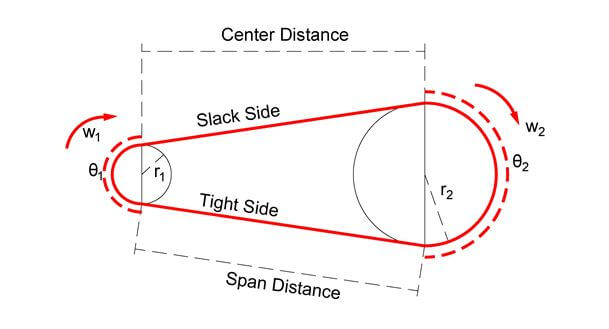
Figure 6: This figure shows the variables for belt drives that will help you to solve the following equations.

The angle of wrap is given as theta 1 and theta 2. These angles are important because they determine the amount of the belt that is in contact with the pulley.

The amount of torque on each of the pulleys can be found with the below equations. Torque is a function of the difference in tensions between the tight and slack side and the radius of the pulley. The larger pulley will have a larger torque and a larger difference between the tight and slack side will have a larger torque.

The ratio of the tight and slack forces is equal to the natural logarithm of the angle of wrap and the coefficient of friction.

Belt drive questions can also revolve around the speed of the two pulleys. The ratio of the speeds of the two pulleys or sheaves is inversely proportional to their diameters.

When you multiply the radius (one-half diameter) by the rotational speed, the result is the linear speed of the pitch line. You can visualize this if you were to imagine a single point moving along the belt. The linear speed of this single point, also known as linear pitch speed, is shown below.

The above equation only works if the rotational speed is in radians per time. If the rotational speed is given in RPM, then RPM must first be converted to radians per minute.

The technical study guide continues with similar discussions on V-belt drives and chain drives.

The topic of shafts and keys focuses on the key, which is a component that is used to connect one rotating component to a shaft. When the key is not inserted, then the rotating components will not be connected. When the key is inserted, then the rotating components will be connected. During this time there will be stresses that will occur within the key. Problems on the FE exam will primarily be on the calculation of these stresses.

There are several types of keys, but the figure below shows the main types of keys. These keys are named after their shapes.

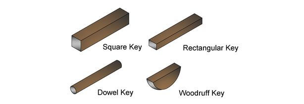
Figure 8: This figure shows different key types.

The different geometry of the keys will cause different stresses to occur within the key. There are two forces that act upon the key, (1) Torsion and (2) Compression. The torsion forces cause a key to shear and the compressive forces cause the key to bend.

The technical study guide covers the shearing forces due to torsion and the compressive forces due to bending. Also included in the guide is a discussion on stress risers aka stress concentration factors and fatigue failure.

12.0 Joining Methods

Bolts, Screws and Rivets

Bolts, screws and rivets are types of fasteners. These types of fasteners are not as strong as the joints created with welding, but are stronger than adhesives. Fasteners are defined as a device that connects two or more components. There are a lot of different types of fasteners but the FE exam luckily focuses only on bolts, screws and rivets.

In preparation for the FE exam, you should be able to calculate the forces and stresses that act upon bolts, screws and rivets. This section will guide you through these calculations. But you should have the correct references to be able to complete these calculations. These references include tables on Bolts, Screws and Rivets that cover the following properties for each type of fastener:

Bolt, Screw and Rivet Properties: Class, grade, tensile area, length, major diameter, minor diameter, tensile strength, yield strength, proof strength, hardness and thread dimensions.

Finally, this section will cover forces in a group of fasteners (bolts, screws and rivets).

A bolt is a type of fastener that passes through a hole in two or more components and is then tightened by a nut on its threaded end. A screw has similar construction, with a head and a threaded end. The difference between a screw and a bolt is in their intended use. Bolts are used to fasten together two unthreaded components with a nut. Screws are used to join components, where at least one of the components is threaded. For example, a screw that is drilled into two pieces of wood joins two threaded components. The screw creates the threads within the wood. A bolt that connects two pieces of wood would require a non-threaded hole. The bolt would be set into the hole, connecting the two pieces of wood. A nut would then be used to tighten the two pieces together.

Figure 5: : A bolt connects two non-threaded components. A bolt is placed at the threaded end of the bolt to secure and tighten the two components together.

The nut is threaded and matched to the bolt. The lifting and lowering torque required to tighten or loosen the nut is similar to the equation shown for power screws. If you encounter a question with a threaded bolt or screw, you may either have to check this section or the power screw section.

The last aspect of bolts is that bolts are removable, similar to screws. Rivets on the other hand are permanent fasteners.

Tension or Clamping Force

The main FE questions will revolve around the purpose of the bolt, which is to clamp two components together. The clamping force causes the bolt to stretch, which means the bolt is undergoing tension. The bolt can also undergo more tension as the joined components undergo more loading. The bolt must be strong enough to resist this tension. The bolt will experience other external loads like moment and shear loads, which will be discussed later.

When a bolt is secured to two components, it produces an initial tension also known as pretension or bolt preload. This is the first force that acts upon the bolt.

The next force is the force due to an external tension load. When a tension load acts upon the two components that are joined together, the amount of external load applied will be divided between the two components and the bolt(s). The equation that determines how much of the load acts upon the bolt and how much of the load acts upon the two components is shown below. In this equation, the initial tension load is added to a fraction of the external tension load or separating force. This fraction is determined by the ratio of the bolt stiffness to the sum of the bolt and clamping stiffness.

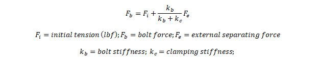
The bolt stiffness and clamping stiffness values are very difficult to calculate. It is highly unlikely that you will have to calculate these values and it is more likely that you will be given the external force that acts upon the bolt. However, just for completeness, the bolt stiffness equation is shown below. The clamping stiffness will vary greatly on the material of the two components selected. The calculation is also much more involved due to the geometry of the bolt in relation to the two joined components.

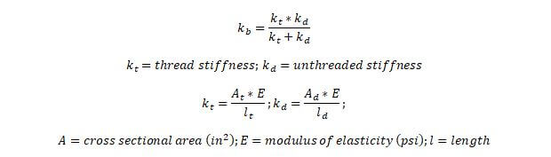
The stiffness of the bolt is a function of the stiffness of the threaded and unthreaded parts of the bolt. The stiffness for each of those parts can be found by multiplying the area of that part by the modulus of elasticity divided by the length of that part.

On the FE exam, you may be asked to calculate the maximum tensile force that a bolt can withstand. This can be found by multiplying the tensile area by the tensile strength of the bolt.

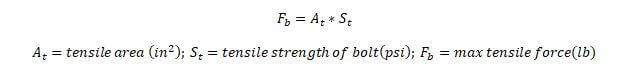
If the tensile stress area is not provided in the tables and the FE exam asks you to calculate the tensile stress area, then you can use the following equation for threaded areas. For non-threaded areas it is simply pi multiplied by the radius squared.

The technical study guide contains the following topics on bolts, screws and rivets:

• Thread Shear
• Fatigue
• Screws
• Rivets
• Concentric Tensile Force on Fastener Group
• Concentric Shear Force on Fastener Group
• Concentric Tensile & Shear Force on Fastener Group
• Eccentric In-Plane Force on Fastener Group
• Eccentric Out-Of-Plane Force on Fastener Group

13.0 Manufacturability

This topic is covered in the practice exam and technical study guide, see the link below.

14.0 Quality and Reliability

In Machine Design, quality assurance and quality control are very important. This topic is generally broad, but in machine design it is focused on the conformity of products. In order to produce quality control in the most efficient manner, quality control charts and techniques were created. Since it would be very inefficient to individually inspect and measure each part and product for perfect quality, the following statistical approaches are used. Calculations for these statistical approaches are time consuming and typically require complex calculators or software. However there are some aspects of quality control that can be tested on the FE exam.

Control Charts

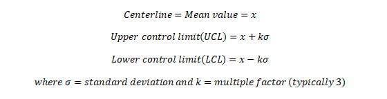
On the FE exam you may be presented with a control chart or a table. Both forms are used to present the level of quality in a production batch. The control chart will measure a certain aspect of the product that needs to be quality controlled. For example, a bolt’s diameter must be measured in order for it to fit within a specific application. Once the bolt diameter is measured within a set of tolerances, it can be labeled as a certain size. The allowable tolerance values are represented by the upper and lower control limits in the equations below.

An example will be shown to walk you through the calculations for mean value and the UCL/LCL values.

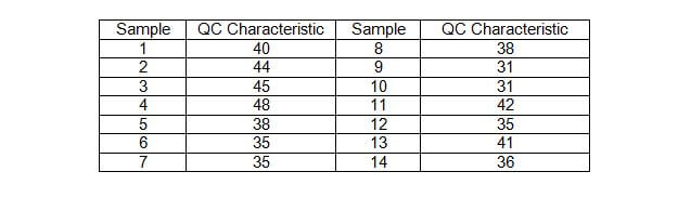
In the above chart, the QC characteristic is a measurement for a specific sample. The mean or average value of the samples is found by adding up all the QC Characteristic values and dividing by the total number of samples which is 14. In this example, the mean or average value is 38.5. The standard deviation is found by adding up the square of the differences between each QC characteristic value and the mean value, then dividing this number by the number of samples. Finally take the square root to find the standard deviation.

The mean and standard deviation can then be used to find the UCL and the LCL. For this example, assume k = 3.

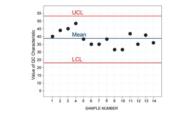
Figure 11: This figure shows the mean and UCL/LCL lines for the table of samples previously shown.

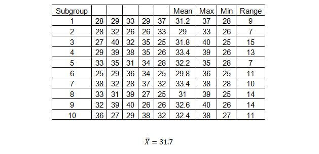
Control Charts with Sample Sizes

The previous section gave you the basics of control charts and introduced terms like mean, UCL and LCL. This section builds upon the basics and introduces the term sample sizes. Sometimes samples are taken in sets/groups of 3 to 10 samples per set or sometimes more. When you take a group of samples, there are two values that you can measure for each group. The first is the mean of that group of samples, the second is the range.

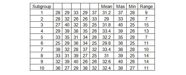
The range is simply the difference between the largest and smallest value within the subgroup.

There are three types of charts that are created to monitor quality control. These charts are the R Chart, X bar Chart and the s-Chart. The R-chart is a plot of the ranges of the subgroups. The X bar chart is a plot of the averages of the subgroups and the s-chart is the plot of the sample’s standard deviations. Luckily the s-chart is much more complex and its equations are more involved, which indicates that the s-chart will most likely not be on the FE exam. Therefore, you should focus on the other two charts. In order to understand these charts you must also understand the following table, which shows the factors for computing the control limits and centerlines for these charts, based on the number of samples. The following guide introduces how the constants on the next table apply to the various charts.

Control Chart Factors

A2: This control chart factor is used to find the UCL and LCL of the averages as a function of the grand mean and the average range.

D4 and D3: These control chart factors are used to find the UCL and LCL of the average range.

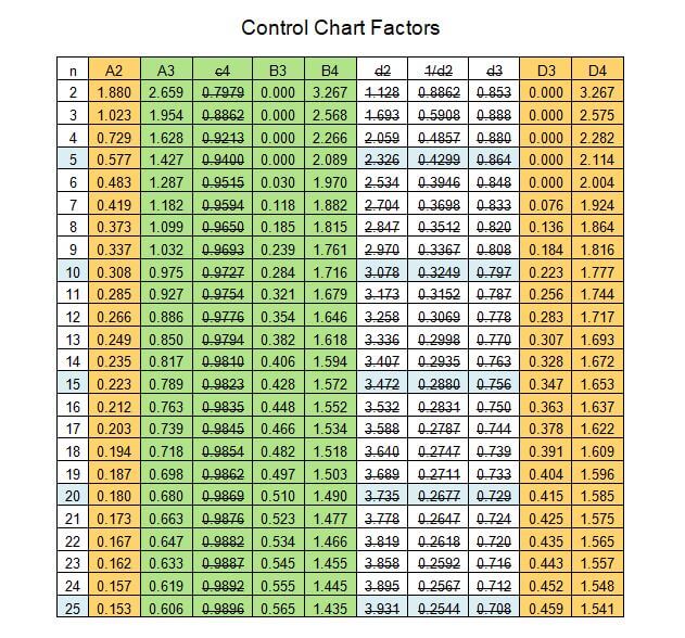
d2 and 1/d2: These two terms are crossed out because these values are only used to determine A2.

d3: This term is crossed out because it is only used to determine D3 and D4.

B3, B4: These terms are used in s-charts to find UCL and LCL.

A3: This term is used to find the UCL and LCL of the grand mean through the use of the average standard deviation.

c4: This term is crossed out because it is used primarily to find A3, through the following equation.

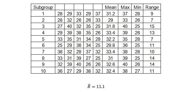
R Chart

The R-chart plots the ranges for the various subgroups and the average (mean) of the ranges for all the subgroups. The average of the example is 11.1.

Next, in order to find the UCL and LCL, you must use the following equations.

You should notice that the sample size is 5, thus the corresponding factors are as shown below:

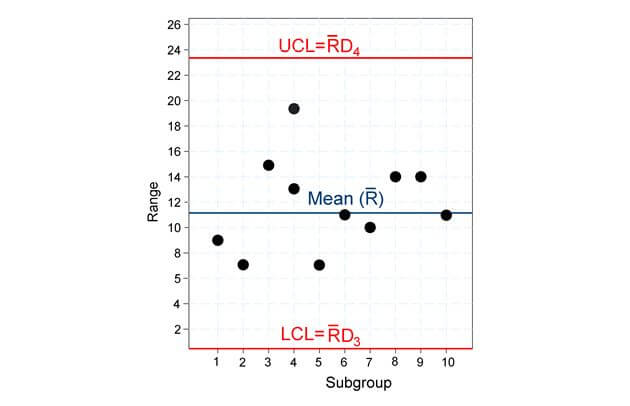
Figure 12: This figure shows the mean range value and the upper control limit and lower control limits based on the control factors and the previous equations.

X-Bar Chart

The X-Bar chart graphically shows the averages of each subgroup. The average of the averages is called the grand average and is shown as, X ̿. This value serves as the centerline of the graph. The upper and lower control limits are found through the following equations.

Next, in order to find the UCL and LCL, you must use the following equations.

You should notice that the sample size is 5, thus the corresponding factor is as shown below:

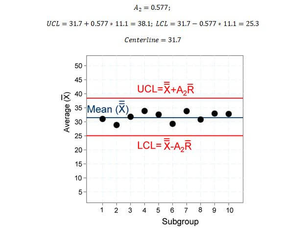
Figure 13: This figure plots the average values for each subgroup. The grand average, UCL and LCL values are also shown with their equations.

s-Chart

The s-chart plots the standard deviation values for each subgroup. The mean of the standard deviations (s ̅) is plotted as the centerline. The UCL and LCL lines are plotted in accordance with the below equations.

Another version of the X-Bar chart can also be plotted with the following equations.

15.0 Hydraulic Components

Hydraulics includes the equipment necessary to do work with liquid. This includes pumps, pipes, pressure vessels, control valves, actuators and connections, as shown in the simple hydraulic system below.

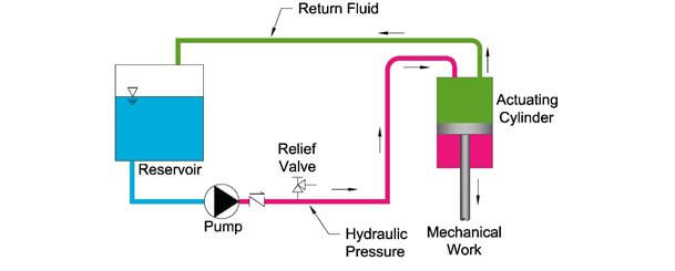
Figure 9: A simple hydraulic system consists of a reservoir that holds the hydraulic fluid, followed by a pump that pressurizes the fluid. The pressurized fluid in pink is then used to power an actuating cylinder to conduct mechanical work. In order to avoid over pressurization, there is a relief valve in the system. The green line shows the hydraulic fluid returning back to the reservoir when not needed.

This topic is covered in the practice exam and technical study guide, see the link below.

16.0 Pneumatic Components

Pneumatics includes the equipment necessary to do work with air. This includes compressors, tubing, pressure vessels, control valves, actuators and connections, as shown in the simply pneumatic system.

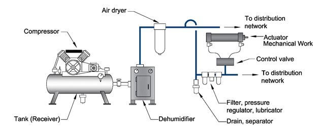
Figure 10: A simple pneumatic system consists of a receiver that holds the compressed gas, followed by a compressor that pressurizes the gas. The pressurized gas then goes through a dehumidifier, air dryer filters and drains, before it finally reaches the actuator. The actuator is used to conduct mechanical work.

The technical study guide covers pumps, dynamic head, net positive suction head, affinity laws, compressor work, actuator cylinder force, cylinder pressure, bulk modulus and hydraulic fluid flow. There is also information on control valuves used in hydrualics and pneumatics.

This topic is covered in the practice exam and technical study guide, see the link below.

17.0 Electromechanical Components

Motors & Engines

Motors and engines are used to transform electricity to mechanical power. A typical FE exam problem would be to size a motor or engine to provide enough mechanical power or horsepower for an actuator, a compressor, a pump, shaft rotation, power screw torque, etc. The typical FE exam skill for motors and engines is being able to convert mechanical power to electricity.

When selecting mechanical equipment, the mechanical engineer must coordinate the power requirements with the electrical engineer. This is done through the following four steps: (1) Determine Mechanical Horsepower, (2) Determine Fan/Pump Brake horsepower, (3) Determine Motor Horsepower and finally (4) Determine Electrical Power.

The technical study guide takes you through this process with examples and diagrams.

18.0 Practice Exam Problems

18.1 PRACTICE PROBLEM 1 – QUALITY AND RELIABILITY

This problem is covered in the practice exam and technical study guide, see the link below.

18.2 PRACTICE PROBLEM 2 – QUALITY AND RELIABILITY

This problem is covered in the practice exam and technical study guide, see the link below.

18.3 PRACTICE PROBLEM 3 - GEARS

A worm gear is mated with a double threaded worm. The worm rotates at 600rpm and has a pitch diameter of 4 inches. If the worm gear has 36 teeth, what will be the rotational speed of the worm gear?

(A) 33 rpm

(B) 46 rpm

(C) 220 rpm

(D) 230 rpm

18.4 PRACTICE PROBLEM 4 – BEARINGS

A manufacturer’s dynamic capacity rating for a ball bearing is 70,000 lbs, based on 90% reliability. If the bearing is under a load of 12,000 lbs and operating in high temperatures conditions, what is the bearing rating life in terms of operating hours? Assume the bearing is operating at 3600 rpm and a life adjustment factor of 0.8 for the high operating temperatures.

(a) 660 hours

(b) 740 hours

(c) 920 hours

(d) 1100 hours

18.5 PRACTICE PROBLEM 5 – GEARS

18.6 PRACTICE PROBLEM 6 - SPRINGS

A helical compression spring has a total number of 20 coils and has square/ground ends. The shear modulus is 15 x 106 psi. The design load is 100 pounds and the spring has a mean diameter of 4” and a wire diameter of 0.25 inches. What is the design deflection?

(a) 2 inches

(b) 6 inches

(c) 10 inches

(d) 16 inches

18.7 PRACTICE PROBLEM 7 – BELTS & PULLEYS

This problem is covered in the practice exam and technical study guide, see the link below.

18.8 PRACTICE PROBLEM 8 - MANUFACTURABILITY

This problem is covered in the practice exam and technical study guide, see the link below.

18.9 PRACTICE PROBLEM 9 - MANUFACTURABILITY

This problem is covered in the practice exam and technical study guide, see the link below.

18.10 PRACTICE PROBLEM 10 – PRESSURE VESSEL

This problem is covered in the practice exam and technical study guide, see the link below.

18.11 PRACTICE PROBLEM 11 – PRESSURE DROP FITTINGS

This problem is covered in the practice exam and technical study guide, see the link below.

18.12 PRACTICE PROBLEM 12 – NET POSITIVE SUCTION HEAD

A cooling tower is located such that the fluid level in the basin is 10 ft above the centerline for the suction of the condenser water pump. The water is at an average temperature of 86 F. The friction loss from the cooling tower basin to the suction of the pump is approximately 15 ft of head. What is the net positive suction head available at the suction side of the pump with a flow rate of 400 GPM?

h_(vapor pressure)=1.4 ft of head

(a) 12.6 ft of head

(b) 17.6 ft of head

(c) 27.6 ft of head

(d) 30.1 ft of head

18.13 PRACTICE PROBLEM 13 – HYDRAULIC COMPONENTS

This problem is covered in the practice exam and technical study guide, see the link below.

18.14 PRACTICE PROBLEM 14 – HYDRAULIC COMPONENTS

This problem is covered in the practice exam and technical study guide, see the link below.

18.15 PROBLEM 15 – JOINING METHODS

This problem is covered in the practice exam and technical study guide, see the link below.