Introduction

Measurement, Instrumentation and Controls accounts for approximately 5 to 8 questions on the Mechanical FE exam. This section covers the following topics, sensors, block diagrams, system response and measurement uncertainty. In the sensors topic, you must be familiar with the types of sensors that are used to measure, strain, temperature and pressure, since these are the properties that are most commonly used in mechanical engineering, unlike the pH and chemical sensors which are also shown in the NCEES FE Reference Handbook. Block diagrams are used to analyze a control system that consists of different functions in graphical format. You must be able to read and simplify these block diagrams for the FE exam. The system response topic focuses on how control systems respond to various inputs like step, ramp and parabolic inputs. This topic will teach you how to determine if a control system will be stable with the Routh test and how to determine the response error.

2.0 SENSORS

The sensors that you need to know for the FE exam are those sensors that convert a physical measurement into an electrical signal. Typically, the physical measurement changes a circuit’s resistance, which in turn changes the measured voltage, assuming that current remains constant. Others change the voltage directly, like in a thermocouple.

2.1 TEMPERATURE SENSORS

There are two main types of temperature sensors that you need to know for the FE exam, (1) Thermocouple and (2) Resistance Temperature Detector.

The thermocouple uses a composite of two dissimilar metals that creates a voltage as a function of temperature. As the temperature increases, the thermoelectric effect occurs and this effect creates a voltage difference between the two sides of the composite. There are wires that are connected to the opposite sides of the composite that measure the voltage. The voltage increases as the temperature of the composite temperature increases.

The resistance temperature detector works off the basic concept that as a metal increases in temperature its resistance decreases. Thus if the current is maintained constant, then the voltage drop through a metal will decrease as the resistance increases, which increases when the temperature decreases. When the temperature increases, the resistance decreases, which decreases the voltage drop.

Figure 1: In a resistance temperature sensor, the metal element becomes more conductive as its temperature increases. This reduces the resistance which decreases the voltage drop.

2.2 STRAIN GAUGE

A strain gauge is similar to the resistance temperature detector. A strain gauge consists of a foil-like element with a circuit running through it. This element is placed on a component that will undergo strain. As the component lengthens, the strain gauge will lengthen as well. This will cause the circuit wires within the strain gauge to become narrow, which will increase the resistance of the strain gauge.

Figure 2: A strain gauge will measure the change in length of a component by measuring the change in resistance of the wires within the strain gauge.

The wires are connected to a Wheatstone bridge to measure the change in resistance. The change in resistance will correspond to a change in length of the component. This change in length can then be used to calculate strain. The ratio between the change in length of the strain gauge and the measured change in resistance is shown as the gauge factor. This gauge factor is pre-measured for each type of strain gauge. Typically the gauge factor is around 2.

Since, the gauge factor is known, you just need to solve for the difference in resistance of the strain gauge. The change in resistance of the strain gauge is indirectly measured through a Wheatstone bridge. The voltage across the Wheatstone bridge is measured as shown in the following diagram. A known voltage is input into the Wheatstone bridge and the output voltage is measured.

Figure 3: In a Wheatstone bridge all of the four locations have the same resistance value.

In a strain gauge, one of the resistors is replaced by the strain gauge. The strain gauge resistance changes as the strain in the component changes. Then the output voltage is measured and the change in resistance is found with the below relationship.

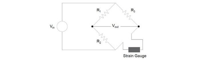
Figure 4: In this figure there is a strain gauge in one of the four locations within the Wheatstone bridge. This is called a quarter bridge. You will notice that in the following equations there is a constant “4”.

All the resistances in a Wheatstone bridge are equal to one another.

You can then plug in the values into the original equation to find the strain.

Sometimes, you must apply multiple strain gauges to a single component to get a more accurate measurement of strain. When this is done, the equation changes as shown below for the different configurations.

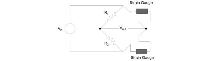
Figure 5: This figure shows strain gauges in two locations of the Wheatstone bridge. This is called a half bridge. You will notice that the constant in the equations below changes from “4” to “2”.

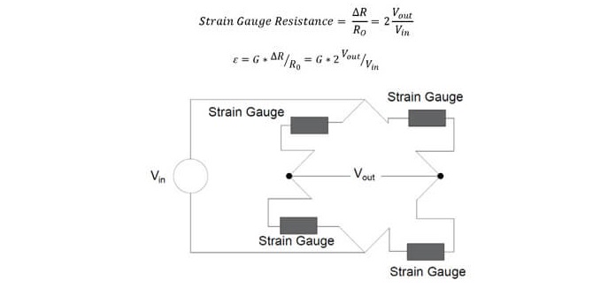
Figure 6: This figure shows a Wheatstone bridge that has strain gauges in each of the four locations. This is called a full bridge and you will notice that there is no constant in the below equations.

2.3 PRESSURE SENSORS

There are two main types of pressure sensors that you should know, (1) Piezoelectric and (2) strain gauge. The strain gauge method uses the previous method to strain as a function of pressure. Then a calculator will convert the strain to a pressure value. The piezoelectric method uses a ceramic or quartz material that strains as a function of pressure. As the material changes shape, it generates an electric field that is measured via wiring and a voltmeter.

3.0 BLOCK DIAGRAMS

Block diagrams are used to diagrammatically show a control system. Each block contains either an input variable or a function that processes a variable.

3.1 FUNCTIONS IN SERIES

If two functions are in series, then the functions can be simplified by multiplying them together.

Figure 7: This block diagram shows an input function “x (t)” entering a control function called “F(t)”. Then the output from F(t) enters another function called G (t). The final output is shown as y(t). The two functions, F(t) and G(t) can be simplified by multiplying the two functions together.

The block diagram of two functions in series can be simplified into the equation format shown below.

3.2 FUNCTIONS IN PARALLEL

If the functions are in parallel, then you can add the two functions.

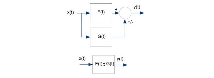
Figure 8: If two functions are arranged in parallel, then the two functions can be simplified by adding the two functions together.

The block diagram of two functions in parallel can be simplified into the equation format shown below.

3.3 FUNCTIONS WITH FEEDBACK LOOP

If the group of functions are arranged to have a feedback loop, then you can simplify the blocks as shown in the below process. In order to simplify the feedback loop, you need to assign an intermediary function B(t).

Figure 9: This figure shows a function x(t) that is processed by function F(t), but the output from F(t) is processed through G(t), which is fed back to the x(t). This is called a feedback loop.

The output is equal to B(t) multiplied by F(t). But you also know that B(t) is equal to y(t)x G(t) + x(t). Then substitute for B(t) into the first equation. The steps are shown below.

This results in the simplification of the feedback loop as shown below.

Figure 10: A feedback loop can be simplified by keeping the original function in the numerator and by adding the product of the original function and the feedback loop processing function.

4.0 SYSTEM RESPONSE

There are two main system response skills that you need for the FE exam. First is determining whether or not the response of a function will be stable or unstable. This is accomplished through the Routh Test. The Routh test determines whether or not all of the roots of a function are negative and real and if they are all negative and real, then the function is stable. The second skill is calculating the steady state error response of a function given various inputs into that function.

4.1 ROUTH TEST

The Routh test is used to determine if all of the roots of a polynomial are negative and real. In order to complete this test, you must follow the below steps.

Step 1: Arrange the polynomial in descending order of power. In this example, x to the fourth is the highest power. If one of the powers is not available, still include it, but the coefficient should be 0.

Step 2: Fill out the top 2 rows of the Routh matrix. You fill out the matrix by starting with the top left cell and including the coefficient into the cell of the highest polynomial. Then input the next polynomial in descending order in the row below. Then go back up to the 1st row, but the second column. Then to the row below and so on and so on. If you have an odd number of polynomials, then the last value will be zero.

Step 3: Fill out the remaining rows. The total number of rows equals the highest polynomial plus 1. So in this example, the number of rows is 5. The remaining rows are filled out by following the pattern shown below. It is like a figure 8. The pattern is a figure 8 that starts at point 1 in the figure below and ends at point 4 below. This shows you how you solve for b1 and b2.

The next figure shows the same pattern but solving for c1 and c2.

The next figure shows the same pattern but solving for d1 and d2.

Step 4: Now that the matrix is complete. The last step is to check whether or not the first column does not change sign. If the first column is all negative or all positive, then the Routh Test has determined that the function is stable.

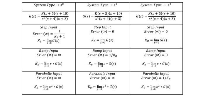
4.2 STEADY STATE ERROR

The steady state error is the error in a function as time approaches infinity.

The steady state error can be found in the FE exam only for systems that are between T = 0, 1 or 2. System types are defined by the variable “n” in the basic equation below.

For example, a system type of T = 0 is shown below.

A system type of T = 1 is shown below.

A system type of T = 2 is shown below.

Most likely, you will be given the equation in the above format and that should tell you the system type.

The next thing you need to know is the input. The inputs can be step inputs (s), ramp inputs (s2) or parabolic inputs (s3).

You can then use the table to find the steady state error given the system type and step input.

5.0 MEASUREMENT UNCERTAINTY

There is one main skill you need to answer problems on measurement uncertainty, which is being able to calculate the propagation of error.

Measurement uncertainty arises from the crudeness of the measurement tools. Tools can only measure accurately to its nearest value. The uncertainty is typically taken as 1/2 the nearest value that a tool can measure. For example, a ruler can measure length to the nearest 1 millimeter, so its uncertainty would be ±0.5 mm. Uncertainty is defined as the value of possible error.

5.1 PROPAGATION OF ERROR

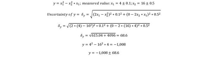
If a measured value has a certain uncertainty or possibility of error, then when that measured value is run through a certain function, then that error will be propagated through that function. The calculation of this propagation is found through the Kline-McClintock method. This method states that the propagation of error is found by taking the square root of the product of the square of the derivative of the function with respect to the measured variable and the square of the uncertainty of that measured variable.

An example is shown below.

This method also works for functions with multiple variables.

An example of this is shown below.

6.0 PRACTICE EXAM PROBLEMS

A characterizing equation is shown below. The variable “C” must be greater than what minimum value in order to ensure the equation stable?

t^3+1000t^2+(C+10)t+100C=0

(a) -9

(b) 0

(c) 9

(d) 1,000

6.2 PRACTICE PROBLEM 2 – THERMOCOUPLE

This problem is covered in the practice exam and technical study guide, see the link below.

6.3 PRACTICE PROBLEM 3 – BLOCK DIAGRAM

Simplify the below block diagram.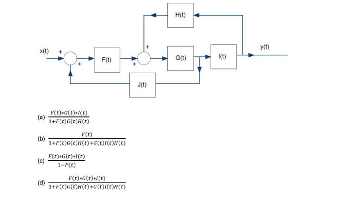

6.4 PRACTICE PROBLEM 4 – STRAIN GAUGE

This problem is covered in the practice exam and technical study guide, see the link below.

6.5 PRACTICE PROBLEM 5 – WHEATSTONE BRIDGE

This problem is covered in the practice exam and technical study guide, see the link below.

6.6 PRACTICE PROBLEM 6 – PRESSURE SENSOR

This problem is covered in the practice exam and technical study guide, see the link below.

6.7 PRACTICE PROBLEM 7 – STRAIN GAUGE

This problem is covered in the practice exam and technical study guide, see the link below.

6.8 PRACTICE PROBLEM 8 – FITS & TOLERANCES

This problem is covered in the practice exam and technical study guide, see the link below.

6.9 PRACTICE PROBLEM 9 – THERMOCOUPLE

This problem is covered in the practice exam and technical study guide, see the link below.