Introduction

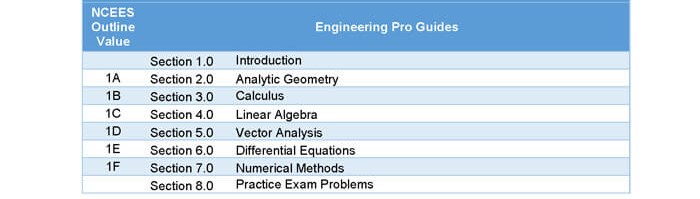
Mathematics accounts for approximately 6 to 9 questions on the Mechanical FE exam. The topics covered in this section include Analytic Geometry, Calculus, Linear Algebra, Vector Analysis, Differential Equations and Numerical Methods. At first glance, these topics seem very vast and daunting. But you should not be worried because you will most likely only need to know the equations that are shown in the NCEES FE Reference Handbook as they relate to Mechanical Engineering.

2.0 Analytic Geometry

Analytic geometry uses algebra to characterize various geometric objects such as shapes, lines and points.

Figure 1: The slope of a line can be found with the difference between the y-values and x-values of two points.

2.1 FIND LINE EQUATION GIVEN TWO POINTS

If you are given two points, then you can follow the below process to solve for the equation of the line. First solve for slope, “m”, where the slope is equal to the change in y over the change in x.

Next, solve for the y-intercept, “b”, using the following equation for a line. To solve for “b”, plug in the value of the slope, “m”, and one of the (x, y) points along the line. Then solve for the y-intercept, “b”.

Finally, replace “b” in the equation and you will have found the equation of the line.

2.2 PARALLEL AND PERPENDICULAR LINES

Another skill you should have is being able to calculate the equation for lines that are parallel or perpendicular to each other. Parallel lines share the same slope.

You can then find the equation of one line that is parallel to another by determining the offset between the lines. Add the offset to the y-intercept of one line to find the equation of the other line.

Figure 2: Parallel lines have the same slope and never intersect.

Perpendicular lines have inverse, negative slopes.

Find the slope of the perpendicular line, then solve for the new y-intercept, “b2”, by substituting one of the (x, y) coordinates on the line.

Figure 3: This figure shows the perpendicular intersection of two lines.

2.3 DISTANCE BETWEEN TWO POINTS

The distance between two points can be calculated with the quadratic equation.

Figure 4: This figure sets up the calculation for the distance between two points.

First, find the total x-distance and the total y-distance. Then you use those values in the quadratic equation.

Figure 5: This figure isolates the previous graph and shows how the distance between two points can be shown as a right angle triangle.

2.4 LOGARITHMIC EQUATIONS

Logarithmic equations are be used in mechanical engineering to describe situations where one variable changes exponentially when compared to another. Logarithmic equations are shown as having the following relationship between exponential functions.

The most important bases are “10” and “e”. The term “e” will be described in the next topic under natural logarithms. If a log function does not have a base specified then you can assume that the base is “10”. The following table shows the result of taking the log of various values of “x”.

The following graph plots “y = log(x)”. It shows that as “x” gets closer to 0, the y value approaches a very large negative number. As x increases the value of y increases slowly. As you can see from the previous table, the difference between each x value gets increasingly large, while the difference between each y value is only 1.

Figure 6: This figure plots the function y = log(x).

The NCEES FE Reference Handbook shows all the applicable logarithmic laws that are used to solve equations with log functions. You should be familiar with how to use those laws on the FE exam. An example of one of those laws is the change of base law, which is shown below.

Change Base: In order to change the original base “b” of a log function, take the log of the value “a” with the new base “n” divided by the log of the original base “b” with the new base “n”.

2.5 NATURAL LOGARITHMIC EQUATIONS

Natural logarithmic equations follow the same rules and laws as logarithmic equations, except the only difference is that the base is “e”. The term “e” is a mathematical constant, founded by Euler. It is approximated as “2.71828”. Natural logarithmic equations are used in the rotational sections of mechanics and with pulleys. The natural log is not written as log base e, but written as ln and the base “e’ is implied.

2.6 TRIGONOMETRY

The main skills that you need to know for trigonometry are the right angle equations and the law of cosines & sines for all other triangles. These skills will help you to determine the angles and lengths of triangles for any situation.

2.6.1 Right Angle Equations

The right angle equations can be used to solve for angles or lengths of a right angle (90 degree) triangle when given either angles or lengths. The pneumonic used to remember these equations is SOH-CAH-TOA, which stands for sine-opposite over hypotenuse, cosine-adjacent over hypotenuse and tangent-opposite over adjacent.

Figure 7: For all right angle triangles, you can use the below equations to solve for the relationships between the angles and lengths of the triangle.

2.6.2 Law of Sines & Cosines Equations

The law of sines and cosines equations can be used to solve for the angles or lengths of non-right angle triangles, when given either lengths of angles.

Figure 8: The law of cosines and sines is necessary to solve some dynamics questions.

The law of sines says that the length of one leg of a triangle divided by the sine of angle opposite the leg is equal to the length of any other leg of that same triangle divided by the sine of the angle opposite that leg.

The law of cosines follow the relationships below, using the same triangle figure above as reference.

2.6.3 Trigonomic Identities

Trigonomic relationships are useful for simplifying and solving equations. A few of the most common identities are provided below. It is not necessary to memorize these. Instead, a comprehensive list of trigonomic identities can be found in the NCEES FE Reference Handbook under the Mathematics section.

3.0 CALCULUS

The calculus required for mechanical engineering include integrals and derivatives. You should be able to find the integral or derivatives for various functions. For example, you may need to integrate the area under a probability curve or find the derivative of a particle position equation to calculate the velocity.

3.1 DERIVATIVES

Derivatives are used to find the slope of a curve and are very useful in dynamics, when you need to find the speed of a component that has a certain displacement function or when you have to find the acceleration of a component that has a certain velocity function.

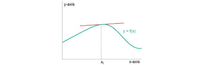
Figure 9: The derivative is the slope at a specific point along a function. This line is tangent to the function curve.

You should be familiar with calculating the derivative for all the functions shown in the NCEES FE Reference Handbook like exponential equations, logarithmic equations, natural log equations, trigonometry equations, etc.

3.2 INTEGRALS

Integrals are used to find the area under a curve and are very useful in mechanics, when you need to find the centroid or area of a shape.

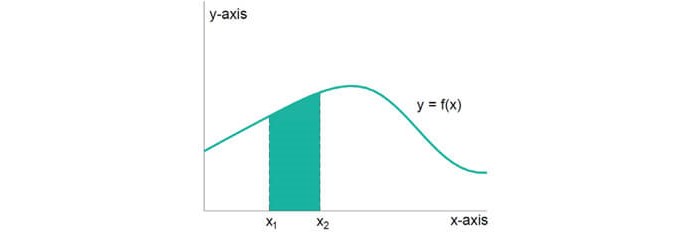
Figure 10: The integral is the area under a curve between two specific points on a function.

You should be familiar with calculating the integral for all the functions shown in the NCEES FE Reference Handbook like exponential equations, logarithmic equations, natural log equations, trigonometry equations, etc.

4.0 Linear Algebra

The linear algebra required for mechanical engineering includes being able to define lines with equations and matrices.

4.1 LINEAR EQUATIONS

Linear equations can be used in statics and dynamics, especially when you want to find the intersection of two functions. In these types of problems you will be given two equations and two unknowns. Then, you can use the skills in linear equations to find the unknown values that satisfy both equations. A very simple example is shown below. The actual questions will most likely be more difficult and will be in the context of mechanical engineering.

First, substitute one of the y-values into the other equation, then solve for x.

Then plug in the x-value to either equation.

The correct answer is, (x,y) = (5/7, 45/7).

Linear equations can extend to multiple unknowns and multiple equations. To simplify the process, matrices are used.

4.2 MATRICES

Matrices are another way to solve linear equations. Matrices are an array of values that can be used to represent multiple linear equations.

For example, the following matrices will represent the below equations.

Rearrange the equation so that the variables follow the same order, constant times x plus constant times y plus constant times z equal to a constant.

The constants for each variable are placed in the first matrix and the variables are placed in the second matrix. The third matrix shows the other side of each equation. The constants in each same row all belong to the same equation and the constants in each column all belong to the same variable.

The values for x, y and z that satisfy all three equations can be found with matrix functions.

The rules for adding, multiplying, taking the transpose, and finding the inverse of a matrix is described in the NCEES FE Reference Handbook. For this test, you should be able to quickly solve for matrices on your calculator. The steps for a typical calculator are shown below. Read through your calculator instruction manual for any variations for your specific model.

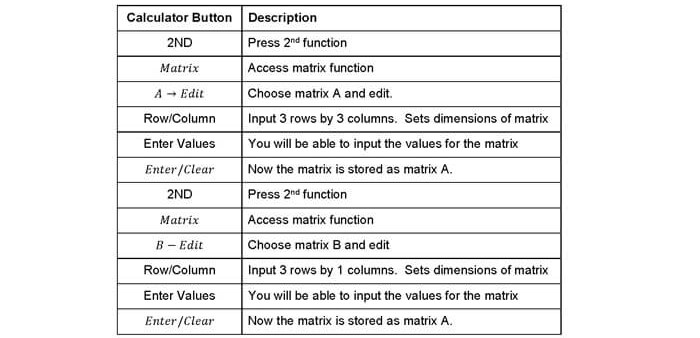
Now that you have input and stored each matrix, the next step is to use the matrices in functions.

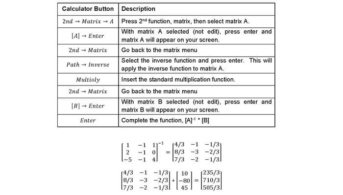
The correct answer is shown below.

You should also be able to calculate determinants, dot products, and cross products of matrices on your calculator.

5.0 Vector Analysis

Vector analysis is used heavily in analyzing forces in Section 7 Statics, Section 8 Dynamics, Kinematics and Vibrations, Section 9 Mechanics of Materials, and Section 15 Mechanical Design and Analysis. One of the main skills that you need is the ability to break down a vector into its x and y components.

Vectors are used to visualize forces and moments in Engineering Mechanics. Vectors describe the magnitude and direction of force or moment. On the FE exam you must be able to translate words or diagrams into force/moment vectors and you must be able to add/subtract vectors and multiply/divide vectors by scalars.

Vectors can either be represented in a rectangular form or a polar form. The rectangular form consists of an x-component and a y-component. These values are used to represent the magnitude in the x and y directions. In real applications, there will also be a z-component, but for the purposes of the exam you most likely will only need the x and y components. The polar form is shown as a magnitude and an angle. The magnitude describes the length of the vector while the angle determines the direction.

5.1 RECTANGULAR FORM

The rectangular form is shown as, x plus the y component. The y component is shown as j and the x component is shown as i.

The rectangular form is used when adding and subtracting vectors and follows the same rules as normal addition and subtraction, where only like terms can be added and subtracted. For example, “Example A” plus “Example B”, is solved with the following process.

The rectangular form can also be understood via a graphical format, where the x-axis represents the real component and the y-axis represents the imaginary component.

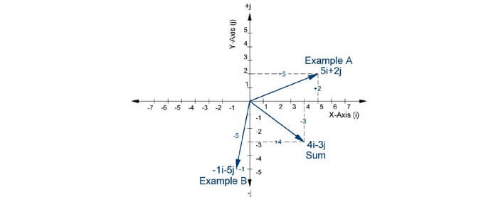
Figure 11: Example “A” vector, example “B” vector and the sum of the two vectors is shown in the above graph.

5.2 POLAR FORM

The polar form is best understood in its graphical format. The format consists of a phasor magnitude at a phasor angle relative to the x-axis.

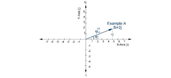
Figure 12: A phasor shown in both polar and rectangular form.

In the above example, the polar form is converted from the rectangular form by using the Pythagorean Theorem to find the radius (i.e. the magnitude) and the inverse tangent to find the angle. The polar form is not typically used for adding or subtracting, but it is used for multiplication and division. When multiplying or dividing two polar forms, you must multiple/divide the radiuses and add or subtract the angles. If the polar forms are being multiplied, then you must add the angles and if you are dividing one polar form from another then you subtract the divisor angle from the dividend angle.

5.3 CONVERTING POLAR AND RECTANGULAR FORMS - CALCULATOR

During the exam, you will need to convert from polar form to rectangular form and vice versa. You will need to convert between the two forms in order to carry out multiplication/division or addition/subtraction. You should be able to quickly convert between the forms with your calculator. This will help to save you time for more difficult tasks during the exam.

You should use the most advanced calculator allowed by NCEES. The calculators allowed by the NCEES are shown below.

• Casio: All fx-115 and fx-991 models (Any Casio calculator must have “fx-115” or “fx-991” in its model name.)

• Hewlett Packard: The HP 33s and HP 35s models, but no others

• Texas Instruments: All TI-30X and TI-36X models (Any Texas Instruments calculator must have “TI-30X” or “TI-36X” in its model name.)

Casio FX-115, Casio FX-991, HP35 and TI-36X are all decent calculators that can do multiple calculation steps without having to use the memory function in the calculator or without having to write down numbers in between steps. However, the Casio and TI models are the cheapest. Past test takers seem to prefer the TI-36X Pro for its interface and its ability to save previous calculations when it is shut off and the Casio FX-991EX ClassWiz for its faster processor and its spreadsheet option. Whichever calculator you decide on using, make sure that you use the calculator during your studying so that you can be well versed in the use of your calculator prior to taking the exam.

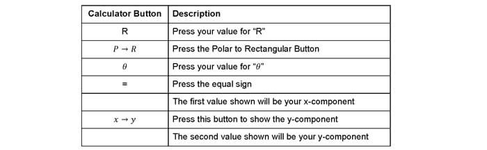
The following are the basic steps in converting from polar form to rectangular form. The above calculators also have the option of adding/subtracting and multiplying/dividing multiple polar or rectangular numbers. Please be sure to learn this skill, because you will use the skill throughout the exam.

Convert Polar to Rectangular xi+yj

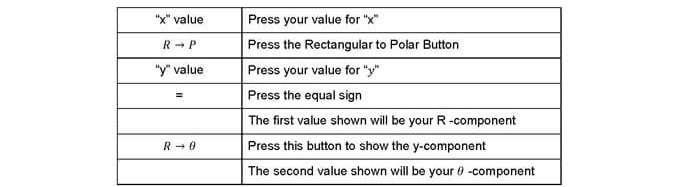
Convert Rectangular (xi+yj) to Polar

The Casio FX-115ES Plus/Casio FX-991EX ClassWiz and TI-36X Pro also has a complex mode which allows you to add/multiply complex numbers in various forms and easily converting the results between rectangular and polar. The stored lines of calculations and the various functions, including matrices and integrals make this calculator one of the favored among test takers.

5.4 VECTOR MATHEMATICAL OPERATIONS

Addition & Subtraction of Vectors: Vectors can be added or subtracted from one another by simply adding or subtracting their real components together and doing the same for their imaginary components. It is very easy to do this when vectors are presented in their Rectangular coordinates, however it is more difficult to do this by hand when the vectors are in polar form. For example, if you are adding 3 and 3j, then the answer is simply 3 + 3j. Another example would be if you were to add the vectors “2+2j” and “4+4j”, then the answer would be “6+6j”.

1st Example: You can complete this problem by inputting the polar vectors and adding them. If you are doing the equation by hand, then you should follow the recommended method by converting polar to rectangular and then adding the like terms to one another (real + real and imaginary + imaginary).

2nd Example: This example is a little less intuitive, but since both vectors have the same angle, they can be added directly or with your calculator. If you are doing the equation by hand, then you should follow the recommended method by converting polar to rectangular and then adding the like terms to one another (real + real and imaginary + imaginary).

3rd Example: In this example, the answer cannot be seen as intuitively, but as long as you either use your calculator to add polar coordinates or convert to rectangular and then add the like terms, then you will be able to complete this problem.

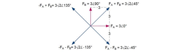
This figure below shows how vectors can be added and subtracted. This figure also corresponds to the first example and it also shows how the answer would change if vectors A and B were subtracted or added.

Multiplication & Division of Vectors: The multiplication and division of vectors is easy for vectors in polar form but difficult for vectors in rectangular form. Your calculator should be able to divide and subtract in both rectangular form, but if you are not familiar with this function on your calculator, then you can also complete this by hand. In order to multiply or divide vectors by hand you must convert the vector to polar form and then multiply or divide the radius of the vectors and then add or subtract the angles. You add the vector angles for multiplication and subtract the vectors angles for division.

1st Example: In this example, the vectors are already in polar form, so you can simply multiply the radiuses and add the vector angles.

2nd Example: Again, the vectors are already in polar form, so multiply the radiuses and add the vector angles.

3rd Example: In this example, the vectors must first be converted to polar and then the radiuses can be divided and the vector angles can be subtracted.

6.0 Differential Equations

Differential equations are used in mechanical engineering to curve fit data. This type of math typically uses software, so it is unlikely that you will have a question on differential equations on the FE exam.

7.0 Numerical Methods

Numerical methods are used with differential equations in mechanical engineering to curve fit data. This type of math typically uses software, so it is unlikely that you will have a question on differential equations on the FE exam.

8.0 Practice Problems

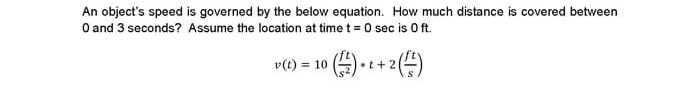
8.1 PRACTICE PROBLEM 1 – CALCULUS

8.2 PRACTICE PROBLEM 2 – CALCULUS

8.3 PRACTICE PROBLEM 3 - CALCULUS