1.0 Introduction

Engineering Economics accounts for approximately 3 to 5 questions on the Mechanical FE exam. As an engineer, you will be tasked with determining the course of action for a design. Often times this will entail choosing one alternative instead of several other design alternatives. You need to be able to present engineering economic analysis to their clients in order to justify why a certain alternative is more financially sound than other alternatives. The following topics will present only the engineering economic concepts that you need for the FE exam and does not present a comprehensive look into the study of engineering economics. For the FE exam you are required to know the following concepts shown in the table below. Applicable equations for these topics can be found in the Engineering Economics section of the NCEES FE Reference Handbook.

2.0 Time Value of Money

2.1 FUTURE AND PRESENT VALUE

It is important that the engineer understand that money today is worth more than money in the future. This is an example of the time value of money. For example, if you were given the option to have $1,000 today or to have $1,000, 10 years from now. Most people will choose $1,000 today, but not understand why this option is worth more. The reason $1,000 today is worth more is because of what you could have done with that money and in the financial world this means how much interest could you have earned with that money. If you took the $1,000 today and invested it at 4% per year, you would have $1,040 dollars at the end of the first year.

If you kept the $1,040 in the investment for another year, then you would have $1,081.60.

At the end of the 10 years the investment would have earned, $1,480.24.

An important formula to remember is the Future Value (FV) is equal to the Present Value (PV) multiplied by (1+interest rate), raised to the number of years.

As an example, what would be the present value of $1,000 10 years from now, if the interest rate is 4%.

Thus in the previous example, receiving $1,000, 10 years from now, is only worth $675.46 today. It is important to understand present value because when analyzing alternatives, cash values will be present at all different times and the best way to make a uniform analysis is to first convert all values to consistent terms, like present value.

Convert all terms to consistent terms.

For example, if you were asked if you would like $1,000 today or $1,500 in 10 years (interest rate at 4%), then it would be a much more difficult question. But with an understanding of present value, the "correct" answer would be to accept $1,500, 10 years from now, because you would only be able to get $1,480 10 years from now, should you accept the $1,000 today, with the current interest rate of 4%. In this example, the $1,000 today was converted to the future value 10 years from now. Once this value was converted, it was then compared to the future value that was given as $1,500, 10 years later.

2.2 ANNUAL VALUE OR ANNUITIES

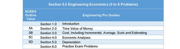
The previous section described the difference between present value and future value. It also showed how a lump sum given at certain times are worth different amounts in present terms, basically the value of a lump sum now is not worth the same in the future. In engineering, there are often times when annual sums are given in lieu of one time lump sums. An example would be annual energy savings due to the implementation of a more efficient HVAC system. Thus, It is important for the engineer to be able to determine the present/future value of future annual gains or losses. For example, let's assume that a solar hot water project, provides an annual savings of $200. Using the equations from the previous section, each annual savings can be converted to either present or future value. Then these values can be summed up to determine the future and present value of annual savings of $200 for four years at an interest rate of 4%.

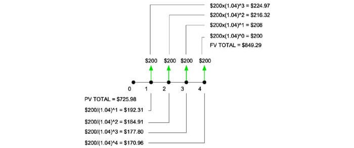
Figure 1: Annual value shown on a cash flow diagram

For longer terms, this method could become tedious. Luckily there is a formula that can be used to speed up the process in converting annuities (A) to present value and future value.

Reverse Equations:

3.0 Cost, Including Incremental, Average, Sunk & Estimating

3.1 AVERAGE COSTS

Average costs is the total cost to produce one unit. It is the fixed and variable costs divided by the total quantity of units produced.

3.2 INCREMENTAL COSTS

Incremental costs are the changes in expenses due to a variation in productions or services. It is associated with costs that are variable, and are used to make decisions on whether the variation is worthwhile. For example, if it costs $10,000 to produce 200 units and it takes $12,000 to produce 300 units, then the incremental cost is $2,000. The $2000 could include costs such as additional material costs, electricity expenses to operate machines, the pay for manufacturing and sales personnel to work additional hours, and advertising costs. It does not include costs that are fixed or do not change with the decision, such as building rent, the initial investment of a production machine, or the cost of personnel healthcare. The business must decide if it is worth the incremental cost to produce additional units. Marginal costs are similar, except it is the variable cost to produce one additional unit.

3.3 SUNK COSTS

Sunk costs are costs that have already been generated and cannot be recovered, such as the purchase of a machine or the payment of a lease. These costs are not included in business decision making processes, since it is already lost and has no effect on the future.

Sunk Costs ($)=Unrecoverable Expenses

Sunk costs can be compared with incremental costs for a business decision making process with the following example.

Example: A facility is determining whether to replace a pump with a more efficient one. The cost for the replacement is the incremental cost, while the cost already incurred for the old pump is a sunk cost and is not used to determine whether the pump should be replaced.

3.4 ESTIMATING COSTS

Cost estimations in mechanical engineering are used to determine the material and installation costs of equipment or systems. Usually this will require the sizing of the equipment based on loads and are used to budget the project. The estimate can then be used in economic analysis to determine the optimal route or to decide whether an investment is worthwhile.

Refer to the “Cost Estimation” section of the NCEES FE Reference Handbook for equations and tables related to cost indexes, capital cost estimation, and scaling of equipment costs. Note that this information is provided under the Chemical Engineering section, but some items are applicable.

3.4.1 Cost Indexes

Cost indexes can be used to convert outdated costs given for a specific year to present day values. A cost index is established and reported by various sources, so the index values should be given to you in the problem. The index is a value representing the average cost of a set combination of goods or services, taken over a set period of time, and calculated for a specific category, such as construction, housing, or food. A cost index can also vary based on an area. Typically a base year is chosen with an index value of 100, then each subsequent or previous year varies with the base. Using this yearly cost index, a ratio can be taken to convert a past cost to a present year value, essentially simplifying the calculations for inflation and deflation for a given category at a given location.

Example: A building in the US is constructed for $1.2 Million in 1978, what is the cost of the building in 2018? The cost index in 1978 and 2018 is 78 and 240, respectively.

Solution: Use the cost index to solve for 2018 values.

The construction cost for the same building is $3.7 million in 2018.

3.4.2 Capital Cost Estimation

Capital costs for mechanical engineering are estimated by the sum of the materials, installation labor, installation equipment costs, and adding a percentage of overhead, taxes, and other indirect fees.

The Capital Cost Estimation tables in the NCEES FE Reference Handbook are meant for chemical process facilities, such as coal or oil, and will likely not be tested. The tables use an estimation factor method, specifically the Lang factors, which are based on sampled data. In these types of problems, the major equipment costs for the facility is given. It is then multiplied by the appropriate factor, between 4 and 6, to find the facility’s total installed cost. The second table lists specific components of the facility and also uses factors. The values listed under the range are given as percentages. Use the total major equipment cost, then multiply by the percentage factor to get the estimated cost for each component.

3.4.3 Equipment Scaling Cost

Finally, the table listed under the “Scaling of Equipment Cost” in the NCEES FE Reference Handbook can be used to estimate equipment of different sizes using an exponential factor “n” that is based on an equipment type.

Example: A 1,000 cfm centrifugal exhaust fan costs $700. What is the estimated cost of a similar fan with 8,000 cfm capacity.

Solution: The table indicates that the exponential factor for a centrifugal fan within the desired capacity range is n=0.44. Solve for the cost of the larger capacity fan with the following equation.

The material cost of the 8,000 cfm fan is approximately $1,748.

4.0 Economic Analysis

Often times the engineer must develop an economic analysis on purchasing one piece of equipment over another. In these calculations, the engineer will use terms like present value, annualized cost, future value, initial cost and other terms like salvage value, equipment lifetime and rate of return.

Salvage value is the amount a piece of equipment will be worth at the end of its lifetime. Lifetime is typically given by a manufacturer as the average lifespan (years) of a piece of equipment. Looking at the figure below, initial cost is shown as a downward arrow at year 0. Annual gains are shown as the upward arrow and maintenance costs and other costs to run the piece of equipment are shown as downward arrows starting at year 1 and proceeding to the end of the lifetime. Finally, at the end of the lifetime there is an upward arrow indicating the salvage value.

Figure 2: Adding salvage value to cash flow diagram.

As previously stated, the most important thing in engineering economic analysis is to convert all monetary gains and costs to like terms, whether it is present value, future value, annual value or rate of return. Each specific conversion will be discussed in the following sections.

Each of the sections will use the same example, in order to illustrate the difference in converting between each of the different terms.

Example: A new chiller has an initial cost of $50,000 and a yearly maintenance cost of $1,000. At the end of its 15 year lifetime, the chiller will have a salvage value of $5,000. It is estimated that by installing this new chiller, there will be an energy savings of $5,000 per year. The interest rate is 4%.

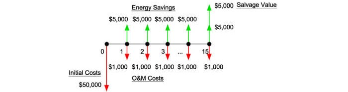
Figure 3: Sample cash flow figure for example problem

Convert to Present Value

What is the Present Value (Present Worth) of this chiller?

The first term, initial cost is already in present value.

The second term, maintenance cost must be converted from an annual cost to present value.

However, we can add the annual energy savings to this amount to save time.

The third term, salvage value must be converted from future value to present value.

Finally, summing up all the like terms.

A negative Present Value indicates that the investment does not recoup the initial investment.

Convert to Future Value

What is the Future Value (Future Worth) of this chiller at the end of its lifetime?

The first term, initial cost is in present value and must be converted to future value.

The second term, maintenance cost must be converted from an annual cost to future value. However, we can add the annual energy savings to this amount to save time.

The third term, salvage value is already in future value.

Finally, summing up all the like terms.

Convert to Annualized Value

What is the Annual Value of this chiller?

The first term, initial cost is in present value and must be converted to annual value.

The second term, maintenance cost is already annualize. However, we can add the annual energy savings to this amount to save time.

The third term, salvage value is in future value and must be annualized.

Finally, summing up all the like terms.

Convert to Rate of Return

What is the rate of return on the investment of $50,000 for the new chiller? The rate of return is a tool used by engineers to describe how profitable or un-profitable an investment is over an equipment's lifetime. The calculation involves determining for a $ investment and a $ monetary gain or loss, what would be the equivalent interest rate. In the previous example, $50,000 is invested in a new chiller and the returns on this chiller are $4,000 a year ($5,000 energy savings minus $1,000 OandM) and a salvage value of $5,000 at the end of the 15 years. For the calculation of rate of return (ROR) or return on investment (ROI), the salvage value is assumed to be $0 only to simplify the problem. The ROR is calculated as what "i" value is required in the below equation to make both sides equal. This approach takes trial and error, unless you have a computer or financial calculator.

First try, i= .04 (4%).

Second try, i= .03 (3%).

Third try, i= .025 (2.5%).

Fourth try, i= .023 (2.3%).

$50,262 is greater than $50,000

Correct answer is approximately, 2.4% ROR. Since, the ROR is less than the interest rate of 4%, this investment is not wise

.

When conducting engineering economic analyses, factor values are used in lieu of formulas. Factor values are pre-calculated values that correspond to (1) a specific equation (convert present value to annual, convert present value to future, etc.), (2) an interest rate and (3) number of years. Looking up these values in a table is sometimes quicker than using the equations and lessens the possibility of calculator error. Looking up these values in a table is sometimes quicker than using the equations and lessens the possibility of calculator error. It is recommended that the engineer use the tables in the NCEES FE Reference Handbook. A summary of the factory values are shown below. which has tables of these factor values. A summary of the factory values are shown below.

5.0 Depreciation

Depreciation is the value that an asset decreases over time. For example, as a building or an equipment gets older, it starts to gradually deteriorate and reduce in useful life over time. Depreciation values can be represented as either a straight line or accelerated form.

5.1 STRAIGHT LINE

Straight line depreciation distributes the depreciation values evenly over the life of the asset. This is the simplest method for calculating depreciation and is represented by the following equation.

For example, a machine is purchased at $100,000 and has a salvage value of $10,000. If the machine has a useful life of 10 years, then the straight line depreciation value is:

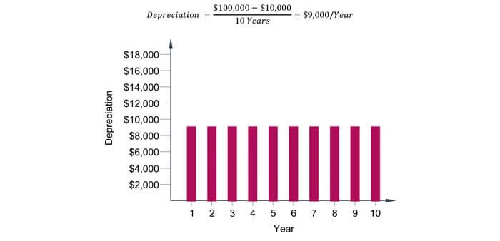
Figure 4: Example of Straight Line Depreciation for an asset with ten years of usable life

5.2 MODIFIED ACCELERATED COST RECOVERY SYSTEM (MACRS)

The modified accelerated cost recovery depreciation system distributes the depreciation to be heavily weighted in the earlier years of the asset’s usable life and less weighted in the later years. In other words, it accelerates the depreciation to earlier in the lifetime of the asset. This system is used for taxes in the United States. It allows for the company to take larger depreciation credits in the earlier years, thereby deferring taxes to later in the asset’s lifetime.

There are two main differences between this depreciation method and the straight line method. First, the depreciation occurs over n+1 years, where “n” is the lifetime of the asset. In addition, there is no salvage value for MACRS depreciation. At the end of the “n+1” years, the asset will have a salvage value of $0.

Depreciation_(year,j) ($ at Year j)=Recovery Rate (%)_(year,j)*Capital Cost ($)

Use the table in the NCEES FE Reference Handbook for the recovery rate based on the recovery period. The same equipment used in the straight line example above ($100,000 initial cost, 10 year lifespan) will have a recovery rate at year 2 of 18%, and a recovery rate at year 8 at 6.55%.

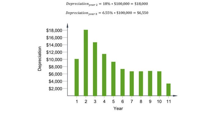
Figure 5: Example of MACRS Depreciation for an asset with ten years of usable life

6.0 Practice Exam Problems

6.1 PRACTICE PROBLEM 1

Background: A client is contemplating on purchasing a new high efficiency pump and motor, with an initial cost of $10,000. The pump has a lifetime of 15 years and is estimated to save approximately $1,000 per year. There is an additional maintenance cost of $300 per year associated with this new pump. The pump will have a salvage value of $0 at the end of its lifetime. Assume the interest rate is 4%.

Problem: What is the annual value of the pump?

(a) -$499

(b) -$199

(c) $199

(d) $499

6.2 PRACTICE PROBLEM 2

Background: A client is contemplating between two separate turbines. Turbine 1 has a life of 25 years, an initial cost of $50,000, an ongoing maintenance/electricity cost totaling $1,000 per year. Turbine 2 has a life of 25 years, an initial cost of $35,000 and an ongoing maintenance/electricity cost totaling $1,500 per year. Assume interest rate is equal to 4%.

Problem: What is the present value of the two turbines?

(a) Chiller 1 = -$65,622 ; Chiller 2 = -$58,433

(b) Chiller 1 = -$91,646 ; Chiller 2 = -$103,455

(c) Chiller 1 = $23,646 ; Chiller 2 = $97,469

(d) Chiller 1 = $12,646 ; Chiller 2 = $103,455