Introduction

Probability and Statistics accounts for approximately 5 to 8 questions on the Mechanical FE exam. Statistics is primarily used in Machine Design for statistical quality control, which is covered under Section 15.0 Mechanical Design and Analysis, under the topics Quality & Reliability. This section focuses on the following NCEES Outline topics, Probability Distributions and Regression Curve Fitting.

Probability Distribution involves applying a mathematical formula to describe the probability of a measured variable occurring at a certain value. This is useful for characterizing the measured output of any mechanical system property when you are taking a sample of a larger number. For example, you measure the weight of 100 products, but this is only a sample of the 10,000 products that are produced. A probability distribution will help to characterize all 10,000 products.

Regression curve fitting involves measuring a variable as a function of another variable, then plotting the data points and assigning a mathematical formula to approximate the function. This is useful in predicting how a change in one variable will affect another.

2.0 PROBABILITY DISTRIBUTIONS

Before you get to probability distributions, you need to understand some of the basic topics in probability like the difference between samples and population, mean, mode, standard deviation. As you go through these topics, you should remember that probability is used in mechanical engineering to measure the reliability of a set of data points.

2.1 MEAN OR AVERAGE

The mean of a set of data points is calculated by summing up all the values and dividing by the total number of data points. The mean is also known as the average.

Sometimes this term can also be called arithmetic mean. An example calculation for finding the mean is shown below for the sample data set.

2.2 MODE

The mode is the measured value that appears the most in a set of data points. In the sample data set from the previous topic, the mode will be “2”.

2.3 MEDIAN

The median is the measured value that occurs in the middle of the data set. The median is found by first ordering all the data points in ascending or descending order, then finding the middle value. If there is no middle value (i.e. there are an even number of data points), then you must take the average between the two middle values.

Data set→{1,2,2, 2, 3,4,10}

The median in the previous example is “2”.

2.4 GEOMETRIC MEAN

The geometric mean is used to give equal weight to a set of data points with high volatility. The geometric mean is found by multiplying the data points and taking the nth root of the product, where n is equal to the number of data points.

On the FE exam, just be careful to read the problem correctly and to make sure you calculate the correct mean. If the question does not specifically state geometric mean, then you can assume that arithmetic mean is required.

2.5 STANDARD DEVIATION

The standard deviation is used to characterize the amount of variation between a set of values. A set of values with a large variation, may lead you to not trust the average of those values or the set of values. A set of values with a small variation, will more likely lead you to trust the average of those values and the set of values itself. Large variations imply volatility, while small variations imply consistency and reliability.

Standard deviation is calculated by first finding the mean, then calculating the difference for each value from the mean. Next, square these differences and sum up the square of the differences. Finally divide by the number of data points, then take the square root of the sum. The equation is shown below.

It is important to note that you can only use this equation when you have a complete set of data points. In the NCEES FE Reference Handbook, this equation is called the standard deviation for a population. This just means that you have the complete set of data points and you are not taking a sample of the complete set of data points. If you are taking a sample of data points, then you must use this formula to calculate the standard deviation.

2.6 PROBABILITY DISTRIBUTION TABLES

The NCEES FE Reference Handbook has a set of probability distribution tables. These tables take the probability formulas and put the results into tables. There are several probability distribution formulas, (1) Binomial, (2) Normal, (3) t-Distribution and (4) x2 Distribution. These tables generally describe the probability of obtaining “x” successes, within “n” attempts or samples, with an individual probability of success equal to “P”. This is often used to predict and test the probability of success, given a number of samples.

2.6.1 Binomial Distribution

A binomial distribution is used when there are only 2 outcomes. Typically in mechanical engineering, these two outcomes are described as success or failure, pass or do not pass, and defective or satisfactory. The following table shows the cumulative binomial probability of success, given “n” independent trials or experiments, “x” successes and “p” individual probability. Say for example you are to flip a coin. The amount of times you flip a coin is “n”, the number of trials. These trials are independent because one does not affect the other. Let’s assume that heads is a success and tails is a failure. The number of heads flipped throughout the trials is “x” the number of successes. Finally, the likelihood of each flip being a heads is 50%, so “p” the individual probability is 0.5. For a set number of trials, n, the binomial distribution will graph out the probabilities of x successes from 0 to n trials. The cumulative binominal probability table includes all probabilities of success from 0 to x. The main objective is to understand how to read and use the Cumulative Binomial Distribution table.

Table 1: This table is read by first identifying the correct column to look at. The columns corresponds to the probability of success for each individual trial or sample. For example, you can assume the individual probability of success is 0.1, meaning that the probability that each product will come out successful is 10%. Next, determine the combination that you want. A combination is the number of successes “x” out of a total number of trials “n”. For example, if you want to know the probability of 0 successes out of 2 trials, then you would find the probability as 0.81. This means that there is an 81% chance that you will select two samples or run two trials and both will be failures, meaning you have zero successes. This table is shown as cumulative, so if you navigate to right below that point you will see a value of 0.99. This means that there is a 99% probability that out of two trials you will either have 0 successes or 1 success. If you calculate the difference between x=1 and x=0, then you will have the probability that there is exactly 1 success, which is 0.99-0.81=0.18 or 18%.

It is very important that you understand the probability of success is cumulative in these tables as you move from x= 0 down to x = 1.

2.6.2 Normal Distribution

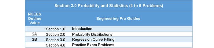
A normal distribution is shown as the figure below. In order to answer these problems, you have to use a different method from the binomial distribution table. The outline of the normal distribution curve may look similar to the binomial distribution at times, but its values are different.

Figure 1: This figure shows the normal or Gaussian distribution. This can also be shown in table form. It shows the probability of a sample’s value appearing a certain standard deviation away from the mean. There is a high probability of the value appearing at the mean, then 1 standard deviation away, then less probability at 2 deviations away and finally least probability at 3 standard deviations away.

This graph can be used as follows. The first way is through the R(x) values. These values tell you the probability that the sample will occur in the range to the right of the (x) value. The (x) value is the number of standard deviations away from the arithmetic mean. This tells you the probability that the sample will occur in the range right of the (x) value of standard deviations away from the arithmetic mean.

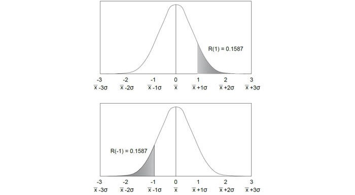
Figure 2: The first way you can look at the normal distribution tables is through the F(x) value. This value is normally used as shown in the top figure. But you can also use it in its inverse format. You can find out the probability that the sample will occur to the left of the negative standard deviations away from the arithmetic mean.

The next way you can use the normal distribution curve is through the F(x) values. These values tell you the probability that leads up to the (x) value when you move from left to right. As you can see this is the inverse of the R(x) values.

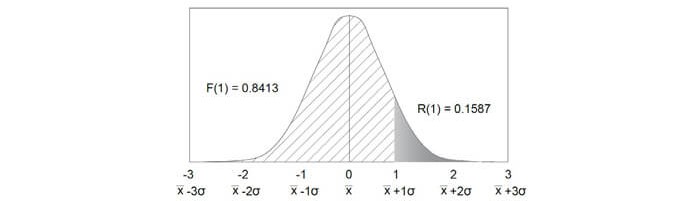
Figure 3: The second way you can look at the normal distribution tables is through the F(x) values. This is the inverse of the R(x) values, meaning that R(x) +F(x) = 1.0.

The third and fourth ways of analyzing the normal distribution is through the W(x) and 2R(x) values. The 2R(x) values is simply found by multiplying the R(x) values by 2. This value tells you the probability that the sample will occur at a value greater than the absolute value of (x) deviations away from the mean. The W(x) values show you the inverse of the 2R(x) values. This describes the probability that a sample will occur at a value less than or equal to the absolute value of (x) deviations within the mean.

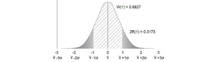
Figure 4: The third and fourth way you can look at the normal distribution tables is through the 2R(x) and W(x) values. The W(x) is the inverse of the 2R(x) values, meaning that 2R(x) +W(x) = 1.0.

2.6.3 t-Distribution

A t distribution is used when there is a limited number of samples within a larger population. It is also used when the standard deviation of the population is not known. The t distribution can be used to estimate the probability distribution of the population given the sample size and the degrees of freedom.

The term degrees of freedom is used to describe the number of independent observations within the sample set. This is shown by the equation below.

DOF=n-1;n=number of samples

In order to use the t-distribution tables, you must first find “t”. The equation for t is shown below.

As you can see from the previous equation you also need to know the population mean. An example of using the t-distribution is when you have a sample of 10 widgets, which have a sample mean of 10. The population mean was previously determined to be 11. The sample standard deviation is 1. The t distribution will give you an idea of the confidence you should have in the population mean.

The t distribution table shows that for 9 degrees of freedom (10 samples -1), alpha is equal to around 0.005.

α=0.005=0.5%

The alpha value means that there was a 0.5% chance that the above sample situation would occur, that 10 widgets would be selected and their sample mean would be less than or equal to 10, given that the population mean is 11 and the sample standard deviation was 1.

Figure 5: When you are using the t distribution tables, remember that the probabilities are cumulative and for a single side, but the curve is symmetric. So the table only shows positive values for t, but you can use that value on the negative side as shown in the example. The table shows that for t=3.127, the probability that the t value will be greater than or equal to 3.127 is 0.005. This also means that the probability that the t-value will be less than or equal to -3.127 is 0.005.

2.6.4 x2-Distribution

An x2 distribution is shown as the figure below. In order to answer these problems, use the same methods as the t distribution, but instead of solving for t, you will most likely be given the x2 value. You can then use the number of samples to determine the degrees of freedom.

DOF=n-1;n=number of samples

Then you should go to the table and find the appropriate row that corresponds to the DOF value. Then navigate to the column with the x2 value. The alpha value at the top will correspond to the cumulative probability that the x2value is greater than or equal to the value selected.

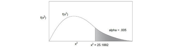
Figure 6: In this figure, 10 degrees of freedom was selected and an x2 value of 25.1882 was found. The corresponding probability is .5%, which means that there is a 0.5% chance that the x2 value could be greater than or equal to the one given.

3.0 REGRESSION CURVE FITTING

Regression analysis is the technique of creating a mathematical formula that describes the relationship between two or more measured variables. Curve fitting for the purposes of the FE exam is the same as regression analysis. In practice, curve fitting and regression analysis are done through the use of a computer software program. Therefore it is highly unlikely that you will be asked to curve fit a dataset by hand. However, you should know how to interpret that data that results from a curve fit.

In the software program, you will have the opportunity to choose the type of curve fit. You can choose a linear fit, square fit or any series of polynomials to fit the data points.

A,B,C & D are constants that are automatically determined by the software

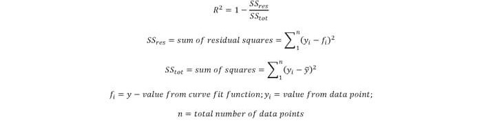
The software program then will output an R2 value. This value is called the coefficient of determination and it describes the fit of the curve as compared to the data points. Please see more in the goodness of fit topic below.

3.1 GOODNESS OF FIT

After you input data into your software program and apply a curve fit to approximate the data with a formula, you will be given an equation and an R2 value.

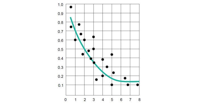
Figure 7: This figure shows data points in black and a mathematical curve fitted to that data.

For a linear fit, the coefficient of determination (R2) value can be found through the below equation. In this equation you need the sum of squares. The sum of squares describe how far apart individual data points are from the mean. The mean is calculated on the right hand side of the equation. There are two sum of squares required for the coefficient of determination, first the sum of squares for the x-values and the sum of squares for the product of the y-values.

You also should understand that for a linear fit, the equation can be found by using the above sum of squares too.

For all other fits, the FE exam will have to give you the following values to calculate the R2 value. However, this equation is not shown in the NCEES FE Reference Handbook, so it is unlikely that the exam will test you on this topic.

4.0 PRACTICE EXAM PROBLEMS

4.1 PRACTICE PROBLEM 1 – BINOMIAL DISTRIBUTION

A product has shown to have a satisfactory probability of 0.5. If there are 10 samples, then what is the probability that only 3 of the samples will pass? The table shown below is a cumulative binomial probability table

.

(A) 0.1%

(B) 1.07%

(C) 5.47%

(D) 11.7%

4.2 PRACTICE PROBLEM 2 – STANDARD DEVIATION

A manufacturing plant produces 500 parts per day. Five parts are sampled and measured with the following tolerances: 1mm, 0.5mm, 0.4mm, 0.4mm, 0.3mm. What is the sample standard deviation of the measured tolerances?

(A) 0.14 mm

(B) 0.25 mm

(C) 0.28 mm

(D) 0.31 mm